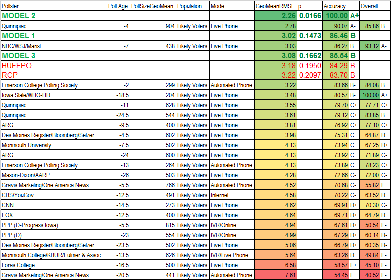
Welcome back! We didn't provide any predictions for the recent Nevada Republican caucus, because there were too few polls on which to base our models. So on we go to the upcoming South Carolina Democrat primary. Both our models forecast blowout victories for Clinton, compared with the poll averages, because of last minute movement towards Clinton. Here are the numbers:
Model 1 - Clinton 75.2%, Sanders 24.8%
Model 2 - Clinton 69.8%, Sanders 30.2%

We thought it would be interesting to provide the probability of each of the remaining 7 presidential candidates achieving the nomination of his or her party. We based a simple model on two criteria: 1) how many delegates has each candidate accumulated so far as a fraction of the total needed to secure a majority; and 2) the current standing in the national polls. Here is the result.

Clinton has the highest probability of achieving her party's nomination. However, her direct competitor Sanders is only about 5 points behind. Trump's probability of winning is a bit lower, but in a much larger field; his probability of winning is more than the second place and third place combined. Of course these numbers will be updated after delegates are awarded in the SC primary. After that, Super Tuesday is make or break for Kasich and Carson.

(Updated Feb. 19) We have been using two models so far with relative success. In Nevada, the predictions are:
Model 1 - Clinton 54.7, Sanders 45.3
There is not enough data to run model 2 in Nevada. In South Carolina, the predictions are:
Model 1 - Trump 28.8, Rubio 21.7, Cruz 17.6, Kasich 11.8, Bush 11.7, Carson 8.4
Model 2 - Rubio 27.7, Trump 26.6, Cruz 17.9, Bush 11.4, Kasich 9.5, Carson 6.9
In model 2, Rubio gets a significant surge due to stronger performance in the last few days, perhaps because of Governor Haley's endorsement.

Let's review our performance in New Hampshire.

Our models slightly underperformed the forecasts of Real Clear Politics and the Huffington Post, because of a last minute fall in support for Rubio; not only did he lose undecided voters, he also lost some of his previous support. However, the cumulative track record of our models is still better than the published averages. That is likely to be tested severely this weekend, so stay tuned. We hope to have forecasts for you next week of the SC Democrats and the NV Republicans.

Above are my forecasts for the outcomes for today's New Hampshire presidential primaries. The model 2 forecasts were so accurate in Iowa that I am publishing only model 2 this time (although I computed model 1 for reference). Noteworthy are a very slight closing of the gap on the Democrat side; and on the Republican side, a last-minute surge for Rubio, a slight surge for Kasich, and collapses for Christie, Fiorina, and Carson. These last 3 candidates will find it hard to go on after today. (NH pollsters have not been asking about Gov. Gilmore, who is at 0% nationally, and won about 0.01% of the vote in Iowa.)

Dr. Carson's campaign has suffered from a lack of attention not consistent with his 4th place position nationally. I noticed a disparity in the number of minutes each candidate was given in the last 3 Republican presidential debates. Dr. Carson received less than half the time given to the most voluble speaker; see below.

Last but not least, the Super Bowl. We were off by only 22 points... The p-value for the observed outcome was .1169, not significant. This reflects the enormous width of the prediction interval, plus or minus 28 points. Back-testing the model, it we got the right winner only once in the last 4 years. It seems that we need a new model! I think I'll wait until after the election in November.

I'll see you after New Hampshire votes are counted to see how our forecast did versus the polls, Real Clear Politics, and the Huffington Post.

OK, it doesn't get any better than this - presidential primaries and the Super Bowl! Let's get started.

The above graph represents a normal approximation to the victory margins achieved by the Carolina Panthers (blue) and Denver Broncos (red) this season. The call: Carolina by 7-8 points. 95% prediction interval: anywhere from a 35-point victory by Carolina to a 20-point victory by Denver. Last year, my model called the correct winner, and the actual victory margin differed from the predicted by just 2 points!

Next, let's call the Iowa caucuses, based on polling data from the last 4 weeks in Iowa.

The data labels show the predicted vote shares by the 3 Democrat and 12 Republican candidates in Iowa; all numbers have a margin of error of 4.5 points. Clinton should achieve a 4.5-point victory over Sanders, while Trump scores a 7.5-point victory over Cruz. Based on the Zipf's law model we discussed in an earlier post, it appears that Sanders is mounting a very strong challenge to Clinton, as are both Cruz and Rubio to Trump.

We hope to analyze the data after the vote, to see which of the polls - or the forecast above - made the most accurate call, as well as to see which types of polling may be more accurate.

Update (later the same day): I have a new model capable of detecting changing direction in the polls. If the new model is correct (and we'll discuss that after the voting), the margin for Clinton will be a mere 1.7 points, while Trump barely edges out Cruz by 2.0 points, in a near 3-way tie with Rubio. Below are the graphs - check back to see which model was more accurate.

OK, one more update, one more model. We'll see tomorrow how this model fares against the other two and the polls and the results.

Voters will start speaking their minds shortly in caucuses and primaries across America. Among the many issues one weighs when voting is a pragmatic one: which candidate is best positioned to win the general election? The answer to that question is complex. For simplicity, we decided to look at the results of national head-to-head polls between the two leading Democrat presidential candidates versus the five leading Republican presidential candidates.

This data was obtained January 28, 2016 from Huffington Post Pollster, which tracks a more comprehensive set of polls than does Real Clear Politics. We chose "More smoothing" to remove noise; we removed polls based on live phone interviews, which seem to be less reliable than other forms of polling, according to a study by Morning Consult; and we removed polls of all adults, focusing on polls of likely voters and registered voters alone. The numbers in the table represent the comparative percent advantage of the Democrat candidate over the Republican candidate.

On average, the Democrats have a 2-3 percent advantage over Republicans. This varies by candidate. The obvious outlier is the Carson-Sanders match-up. This is probably an artifact of the fact that only one poll made it through our filters, so the point estimate is probably unreliable.

On average, there is little difference between the performance of the two Democrat candidates. The Republican candidates are ordered in the table in order of increasing strength. Trump has the best average performance against the Democrat field. In turn, Clinton has a better chance of beating Trump than does Sanders. See the chart below.

A linear model of the above data suggests that Trump is the strongest Republican presidential candidate, while there is not much substantial difference between the Democrat candidates; see below.

We begin with the candidate power rankings. However, we change the vertical scale compared to last time we discussed the subject; now it measures distance between logits rather than between the raw poll numbers.

Only 4 candidates are above water: Trump, Clinton, Cruz, and Rubio. Sanders, Carson, and Bush are close to break-even. It is hard to consider the other candidates as viable. (Gov. Gilmore is not shown on this graph; he would appear down at negative infinity.)

We consider whether Zipf's law, or some power law, as discussed in an earlier post, could apply to the odds ratios for the candidates in their respective races.

The fit is fairly good in each party, and becomes even better when the trailing candidates (O'Malley, Santorum) are removed.

The expected performance of the leading candidate is given below.

If Zipf's law holds for odds ratios in a 2-person race, the leader should poll about 58.6%. In a 3-person race, it's 46.8%; in a 4-person race, it's 40.9%; and in a 5-person race, it's 37.2%.

Lastly, we analyze the distribution of the 22 national polls in the Republican presidential race conducted entirely during December. We focus only on the 6 top candidates. A biplot is shown below.

There are several interesting items to observe. One is that Trump is the only candidate who has negative correlations with each of the other 5 (the correlation matrix shows this), suggesting Trump is rather distinctive in the race. Another is the appearance of two axes dominating the picture: a Trump-Rubio axis (outsider vs. establishment?) and a Cruz-Carson axis (choices for social conservatives?). We also can perceive poll 21 as a distinctive outlier.

The Democrat presidential race does not offer much in the way of statistical challenges. It has become essentially a 2-person race, for the moment. If that should change, we will analyze it.

The Switkay USA Economic Vitality Index increased 3.30 points to reach a level of 83.65 for the 3rd quarter of 2015, its highest level since the 2nd quarter of 2009.

One of the big drivers of the index in the 3rd quarter was an upward spike in the trade-weighted value of the US dollar of about 3.5%. This may have reflected an anticipation of an increase in interest rates by the Federal Reserve Bank, something that did finally occur in December.

Further, the U6 underemployment rate fell significantly, from 10.7% in the 2nd quarter to 10.2% in the 3rd quarter. However, concern remains over the unusually high U6/U3 ratio, reflecting a higher usage of part-time workers than previously; the fact that Gallup's survey of underemployment reports numbers more than 4% higher than the Labor Department's; and the labor force participation rate of 62.5%, the lowest level since the 3rd quarter of 1977.

The velocity of the M2 money supply is 1.490, the lowest level in the 42+ year history of this dataset; this is an ominous sign for the economy.

The Switkay USA Economic Vitality Index is a function of the following variables:
·         real gross domestic product per capita;
·         total Federal debt as a percentage of gross domestic product;
·         the U6 unemployment rate (including those working part-time who would prefer full-time work);
·         mean weeks of unemployment;
·         average hourly earnings, production and non-supervisory employees, private;
·         US population;
·         the civilian labor force participation rate;
·         the consumer price index, all urban consumers;
·         the velocity of the M2 money stock;
·         the real trade-weighted exchange value of the US dollar (broad index);
·         real net worth of households and non-profits.

It is updated at the end of every quarter, when data for the previous quarter become finalized. We use the word real to mean inflation-adjusted. All data is taken from FRED, the research service of the Federal Reserve Bank of St. Louis. The index is normalized so that its median value in the years 1973 to 2008 is 100.

As campaign season gets underway, inquiring minds want to know: does partisan control in Washington, DC have an effect on economic performance? This question has been asked before, using varied sets of variables, and the answers have varied accordingly. Lattice Insight has been publishing the Switkay USA Economic Vitality Index at the end of every quarter, when finalized data becomes available for the previous quarter. The components making up the index can be tracked back to the beginning of 1973, but they are not all available any earlier.

Partisan control in Washington falls naturally into 2-year time blocks: odd-numbered years followed by even-numbered years constitute one congress, between successive congressional elections. From 1973 to 2014 we have 21 such 2-year periods. In each, the White House was controlled by one of the two main political parties. Congress was controlled by one of the parties, or else control of the two houses was split. (The analysis could be refined further by examining the effect of partisan control of each house; however, control of the Senate and of the House have a moderate positive correlation, and there were too few cases of split control to justify such a division.)

The graphs above show the average performance of the Switkay USA Economic Vitality Index as a function of partisan control of the White House and of the Congress for each of the 21 2-year periods, with Democrat control on the left side of the graph and Republican control on the right side. Republican control of each branch appears to produce a positive effect on the index, and this effect is more pronounced for Congress than for the White House.

In a model including both White House and Congress, control of the White House is almost but not quite significant (p = .0668) in the presence of congressional control; control of Congress remains significant (p = .0223) even in the presence of control of the White House. Thus, as the graphs above suggest, control of Congress has more impact on the economy than control of the White House. The model including these two predictors has an R-squared of .3309, meaning partisan control can explain about 33% of the variability of the economic index. Contrary to popular opinion, there is no significant effect with divided control (p = .8831), in which it has been suggested that the economy benefits from having one party in the White House and another controlling Congress.

The 21 2-year periods are divided into 6 categories, based on control of the White House (D or R) and control of Congress (D, split, or R). The best average value for the index was 125.84, under a Republican president and a Republican Congress (2003-2006). The worst average value for the index was 64.74, under a Democrat president and split Congress (2011-2014).

How are the presidential candidates doing in the polls? Here is one way to visualize it. The rankings utilize the latest value of the smoothed average of all polls published on the Huffington Post, a more inclusive average than that published by Real Clear Politics. Each candidate is compared to the average poll share per candidate; this is 14.3% (100%/7) for the Democrats (in red), and 6.7% (100%/15) for the Republicans (in blue).

Since Biden is included in all polls, he is included in the denominator of the above fraction. If Biden is not included, the standard of comparison would be 16.7% (100%/6) for Democrats, dropping each Democrat candidate 2.4%.

Clinton and Trump hold commanding leads for the time being, although Sanders and Carson are surging. See however my previous post on Zipf's law.

The graph suggests that the lowest ranking four Democrat candidates, and the lowest ranking five (or even nine) Republican candidates could be dropped from future debates without disappointing too much of the public. These candidates are supported appreciably less than the average within their respective parties.

If you enjoy data and politics, there's little more fun than polls. The horse race in the primaries is a field ripe with statistics, which can shed light on the relative performance of the individual candidates, particularly the leaders in each party.

Zipf's law arose in linguistics, but has found applications in other areas. Zipf studied the relative frequencies of words used in a language, like English, and found that the 2nd most frequent word is used about 1/2 as much as the most frequent word; the 3rd most frequent word is used about 1/3 as much as the most frequent word, and so on. That is, word frequency is inversely proportional to word rank. A similar pattern occurs examining the populations of a country's cities, and other agglomerations.

It appears that a version of Zipf's law applies to the popularity of the presidential candidates. The leftmost dot in each graph represents the leader (currently, Trump and Clinton). The relatively large value of R-squared tells us that the model has very good predictive power.

If Zipf's law applied exactly, the coefficient of x in the regression equation would be -1 (since the graph is essentially plotted on log-log paper). The steeper slopes of the lines above is a result of the downward pull on the right side of the graphs by the lowest-ranked candidates, who are performing worse than Zipf's law would predict. It seems rather safe to predict that these candidates (Gilmore, Graham, Pataki, Jindal, and Santorum; and Chafee, Webb, and O'Malley) are unlikely to last, if only for financial reasons. When these candidates are removed from the dataset, R-squared moves closer to 1 (better predictive power), and the slope of the line moves closer to -1 (Zipf's law). (The graph doesn't include a point for Gilmore, whose poll numbers are roughly 0%, thus off the chart.)

If Zipf's law holds, the leading candidate should be polling around 100%/H_n, where H_n = 1 + 1/2 + 1/3 + ... + 1/n. (When n is large, 1/H_n can be approximated conveniently by 1/(.5772+ln (.5+n)); see the graph below.) Trump and Clinton can be expected to poll around 30% and 41% respectively; the actual numbers are 34% and 44%, a good approximation. The leading candidate should not be expected to pass 40% until there are only 6 candidates left in the race - if Zipf's law describes voter preferences accurately.

This is especially interesting because Trump's poll numbers are close to what would be expected in a 10-person race - exactly what we would have if the bottom 5 Republicans dropped out. The ceiling that some commentators attribute to Trump may be a paper ceiling through which he can rise as the other candidates drop out. In contrast, the Democrat race has only 3 viable candidates, in which case Clinton should be polling around 54%. Her relative weakness may indicate an uneasy electorate.

The Switkay USA Economic Vitality Index increased 2.34 points to reach a level of 80.35 for the 2nd quarter of 2015, its highest level since the 2nd quarter of 2009.

Unemployment is one of the key components of the index. We use data supplied by the Bureau of Labor statistics. We note however that the Gallup estimate of U3 unemployment is about 1% higher than BLS, and Gallup's estimate of U6 (underemployment) is about 3% higher than BLS.

The civilian labor force participation rate remains near a 36-year low. The velocity of the M2 money supply remains near historic lows. Mean weeks of unemployment is at its lowest level since 3rd quarter, 2009. Real GDP per capita remains below its peak in 4th quarter, 2014.

The Switkay USA Economic Vitality Index is a function of the following variables:
·         real gross domestic product per capita;
·         total Federal debt as a percentage of gross domestic product;
·         the U6 unemployment rate (including those working part-time who would prefer full-time work);
·         mean weeks of unemployment;
·         average hourly earnings, production and non-supervisory employees, private;
·         US population;
·         the civilian labor force participation rate;
·         the consumer price index, all urban consumers;
·         the velocity of the M2 money stock;
·         the real trade-weighted exchange value of the US dollar (broad index);
·         real net worth of households and non-profits.

It is updated at the end of every quarter, when data for the previous quarter become finalized. We use the word real to mean inflation-adjusted. All data is taken from FRED, the research service of the Federal Reserve Bank of St. Louis. The index is normalized so that its median value in the years 1973 to 2008 is 100.

A friend asked me about a recent blog post of mine (see below) discussing real GDP per capita. He found the graph a bit hard to read. Above, I have created a new graph in which we see percent change in real GDP per capita for each year over the previous year, 1948-2014, shown with individual bars (green for increase, red for decrease). The wavy curve smooths this data still further into a trailing 4-year moving average, corresponding to the length of a presidential term. For comparison, the median annual percent change in real GDP per capita from 1948-2014 is +2.2%.

Real GDP per capita is one of the key ingredients of the Switkay USA Economic Vitality Index, posted at the end of each quarter, using the final numbers for the previous quarter. While most politicians prefer to focus on raw GDP numbers, these must be adjusted both for the increase in prices (real) and the increase in population (per capita), to get a sense of overall well-being, in just the same way that unemployment rates must be adjusted for part-timers who need full-time work (U6) and the labor force participation rate.

As we await the turmoil in global markets subsequent to the Greek debt bailout referendum, I thought it would be interesting to compare the danger of a default by Greece to that of other countries. What danger do other countries' debts pose to the global financial system?

The model I created makes use of the following variables: 1) credit ratings by Standard & Poor's, Moody's, and Fitch; 2) public debt as a fraction of GDP; 3) total external debt. 1) quantifies the risk of default; 2) quantifies the debt ratio; 3) quantifies the magnitude of external debt. The results are scaled so that the United States of America has a value of 1.00.

The results imply that we should be as concerned about Japan and Italy as much as we are about Greece, with Spain, Ireland, and Portugal not far behind. Although these countries have better credit ratings than Greece, the magnitude of debt involved is much larger, and particularly in the case of Japan, the debt ratio is enormous: about 2.32, far higher than Greece's 1.75.

The Switkay USA Economic Vitality Index increased 4.35 points to reach a level of 78.01 for the 1st quarter of 2015, the highest level of the index since the 3rd quarter of 2009. This came despite a decrease in real GDP per capita of 0.8%. In addition, M2 velocity was at its lowest recorded level of 1.500.

Two factors improved notably during the 1st quarter. The trade-weighted value of the dollar rose nearly 5%, perhaps due to quantitative easing in Europe. Also, mean household net worth increased a bit more than 2%.

The Switkay USA Economic Vitality Index is a function of the following variables:
·         real gross domestic product per capita;
·         total Federal debt as a percentage of gross domestic product;
·         the U6 unemployment rate (including those working part-time who would prefer full-time work);
·         mean weeks of unemployment;
·         average hourly earnings, production and non-supervisory employees, private;
·         US population;
·         the civilian labor force participation rate;
·         the consumer price index, all urban consumers;
·         the velocity of the M2 money stock;
·         the real trade-weighted exchange value of the US dollar (broad index);
·         real net worth of households and non-profits.

It is updated at the end of every quarter, when data for the previous quarter become finalized. We use the word real to mean inflation-adjusted. All data is taken from FRED, the research service of the Federal Reserve Bank of St. Louis. The index is normalized so that its median value in the years 1973 to 2008 is 100.

What would the United States Senate look like if Senate seats were allocated in proportion to states' areas, rather than the equal allocation we have today? The map above shows the result, using the Adams method of allocation.

In the Adams method, every state is guaranteed at least one Senate seat, even though it may constitute considerably less than 1% of the total area of the United States. Consequently, larger states like Alaska lose a bit of representation; Alaska constitutes more than 16% of the area of the US, but only gets 12 Senate seats.

Eight states see their Senate representation increase to more than 2 seats; 21 states stay the same; and 21 states lose representation, going down to one senator. Since a Constitutional amendment can be blocked by 13 states, the map above is unlikely to become reality.

What purpose would be served by such an allocation? Recall that in American history, some states have been formed out of other states. For example: Delaware was part of Pennsylvania during the colonial period; Maine was a colony of Massachusetts; Vermont was part of New York; West Virginia seceded from Virginia; etc. More to the point, Californians recently considered a proposal to partition the state into 6 new states.

Any time a state divides, the combined representation of the new states in the House of Representatives will remain about the same, because it is proportional to population. However, the new states would get two senators each, increasing the proportion of their combined representation in the Senate. Thus the Constitution provides an incentive for states to split. Texas has 254 counties, more than any other state. If all the counties chose to become independent states, they would together control the Senate.

By choosing to allocate senators by area, rather than equally, we remove the constitutional incentive of states to split (although they may still wish to split for other reasons).

How do we know whether we're really economically miserable? The official definition of a recession is two or more consecutive quarters of negative GDP growth. As long as GDP grows by even one dollar during the quarter, that interrupts any recession that might be taking place - officially speaking.

However, reality is more complex. That one dollar growth in production does nothing to improve the well-being of people if prices and/or population have risen during that quarter - and usually they both do increase. A 0.1% increase in your income is a decrease in practical terms if prices have risen by 1%, or if that income is shared by more people.

The graph above shows data downloaded from FRED, the research arm of the St. Louis Federal Reserve Bank. The blue curve is the annualized percent change in raw GDP - the official number, reported by the media. The orange curve is the much more important number, adjusted for price increases and population increases. According to the orange curve, the 2008-2009 recession was four quarters long, not three. 2011Q1 and 2012Q4 were contractions as well according to the orange curve.

As far as we know at this time, we are not yet in a recession. The second quarter will shed more light on this question.

Suppose you drew a random sample from a population. How large could we expect the sample's minimum and maximum to be? Obviously, the sample's minimum and maximum would change every time we drew the sample, but if we drew samples repeatedly, we might expect to see predictable patterns.

In fact, this is the case, and the minimum and maximum are just the two extreme members of the order statistics. The median is also a well-known order statistic, when the sample has odd size. The distributions of all order statistics are known.

If we wanted to determine whether a sample is likely to have been drawn from a normal distribution, for example, we might compare the numbers that were actually observed to the expected values of the order statistics. Too large a departure, and we might suspect that the observations are unlikely to have been drawn from a normal distribution.

This question is often judged by examining a Q-Q (quantile-quantile) plot, or less frequently a P-P (probability-probability) plot. These in turn depend on judgments as to where the order statistics should be plotted. This issue is the unsettled question of plotting positions. There are several plausible formulas for plotting positions that are commonly used. Most have the form Phiinv[(k-a)/(n+1-2a)], where 0<=a<1, k is the index of interest, n is the sample size, and Phiinv is the probit function, the quantile function for the standard normal distribution (and inverse to the cdf of the standard normal). There are strong arguments in favor of a=0 and a=1/2.

A popular estimate (Blom, 1958) of the order statistics of a sample from a normal population makes use of a=3/8. But it turns out this is a somewhat sloppy approximation of the accurate estimate (Elfving, 1947) in which a=pi/8. The approximation depends on the belief that 3 is sufficiently close to pi!

I discussed this question in a post on StatsExchange. Read the original question and the answers here:
http://stats.stackexchange.com/questions/9001/approximate-order-statistics-for-normal-random-variables/152834#152834

It's the question without an obvious answer in cluster analysis: into how many clusters should we group our data? You are lucky if the data groups into a small number of visible, compact clusters that are clearly distinct from one another. Usually the choice is ambiguous, often depending on the clustering method used.

I am a big fan of Ward's method of clustering. The dendrograms associated with Ward's method lend themselves to fairly obvious recommendations for the number of clusters, because the higher branches tend to be the longest, especially in comparison to dendrograms arising from other agglomerative hierarchical clustering methods. (In technical terms, dendrograms arising from Ward's method tend to have larger agglomerative coefficients, closer to 1, compared with complete linkage [2nd best], average linkage [3rd best], and single linkage [the worst].)

The Calinski-Harabasz pseudo-F statistic tries to explain the most variation between clusters using the fewest clusters, employing a formula that suspiciously resembles an F-statistic. When the data is multivariate normal and the clustering method is Ward's, the pseudo-F statistic is in fact an F-statistic!

Typically we try to maximize the pseudo-F statistic. For one dataset I studied recently, the maximum occurred at k = 5 clusters, as shown in the graph above, with k = 8 a close second. The dendrogram reveals that 5 clusters and 8 clusters are natural choices for this data.

But when the pseudo-F statistic is in fact an F-statistic, an alternative is to determine the p-value for the F-values above, and choose the number of clusters that minimizes p, giving us the most significant value of k. In the graph below, the partitioning of variance among 8 clusters is more significant than among 5 clusters. (Horizontal lines on this graph of log p show the location of p = .05 [upper] and p = .01 [lower].)

I originally addressed the issue of stock performance prediction in a post on March 13 of this year. This update takes note of an improved model which now can predict 16.3% of the variability in stock prices. Put another way, the correlation between observed stock performance and that predicted by the model, as shown in the graphic above, is about .404, a major improvement on the previous model. The current model is based on just 7 variables that are available from public sources such as financial websites.

The model is validated in various ways. We note first that all variables remaining in this model are highly significant (p < .000002). Also, residuals are mound-shaped and symmetric (though not quite normal), and Cook's distance is within acceptable bounds. Finally, cross-validation was employed, yielding satisfactory results.

Don't worry if you don't follow the technicalities. The point is that the model is statistically sound, assuming the validity of the original data (which does constitute a somewhat biased sample).

Past performance is never a guarantee of future results. The nature of statistics is such that I can't tell you the exact price of your favorite stock one week from today. But given a large enough set of stocks, and a long enough period of time, this model predicts that stocks with certain characteristics will perform better, on average.

The Switkay USA Economic Vitality Index for 2014, 4th quarter is 73.66. This represents an increase of 2.29 from the previous quarter. The index is continuing to rebound slowly from its recession low of 58.21 in 2011, 3rd quarter. The index now stands at its highest level since 2009, 3rd quarter.

The Switkay USA Economic Vitality Index is a function of the following variables:
·         real gross domestic product per capita;
·         total Federal debt as a percentage of gross domestic product;
·         the U6 unemployment rate (including those working part-time who would prefer full-time work);
·         mean weeks of unemployment;
·         average hourly earnings, production and non-supervisory employees, private;
·         US population;
·         the civilian labor force participation rate;
·         the consumer price index, all urban consumers;
·         the velocity of the M2 money stock;
·         the real trade-weighted exchange value of the US dollar (broad index);
·         real net worth of households and non-profits.

It is updated at the end of every quarter, when data for the previous quarter become finalized. We use the word real to mean inflation-adjusted. All data is taken from FRED, the research service of the Federal Reserve Bank of St. Louis. The index is normalized so that its median value in the years 1973 to 2008 is 100.

The change in the index's value for the 4th quarter of 2014 was driven most strongly by a 4% increase in the real trade-weighted exchange value of the US dollar (broad index). This could be due to an anticipation of a rate increase by the Federal Reserve Bank, or by quantitative easing in Europe, among other reasons.

The U6 unemployment rate declined slightly for the quarter, but the labor force participation rate was unchanged, near 37-year lows, and mean weeks of unemployment increased for the first time in more than a year.

Word clouds are a clever way to visualize the results of text mining. The image above is based on a combination of the texts of the United States Declaration of Independence and the United States Constitution.

So-called "stopwords" are removed from the text. This includes common functional words like articles, prepositions, pronouns, and forms of the verb "to be". The remaining words are depicted with the most frequently occurring words shown as the largest.

Everyone wants to know how to pick a winner in the stock market. What should you look for? I analyzed a dataset created by Stephen Jones, of String Advisors, and Chris Mayer, of Agora Financial's Capital and Crisis: http://agorafinancial.com/publication/fst/

Their dataset contained dozens of variables for hundreds of companies over decades of time. That's a lot of data!

My model suggests you can predict about 12.76% of the variability in the total return of a stock by looking at some of the well-known ratios involving the stock's price - but these ratios play an unexpected role in the formula. Put another way, the correlation between the observed returns and those predicted by my model is about .357, as shown in the image above.

This is only the beginning of a fascinating project. Stay tuned!

You have an enormous set of data: thousands of observations and dozens of variables. How do you locate outliers - possible mistaken data, or problems, or opportunities?

Multivariate statistics gives us the tools to discover these outliers. The above image depicts 2697 observations in 73 variables. The potential outliers are clear in this diagram.

In my analysis of the monthly report from the US Bureau of Labor Statistics, I find it useful to combine 1) the labor force participation rate (measuring the fraction of adults who are working or looking for work), with 2) the U6 unemployment rate, which counts not only the unemployed in the more widely quoted U3 rate, but also long-term unemployed and those working part-time who would prefer full-time work. This combination tells us what fraction of the adult population has full-time work.

The image above covers the period January, 1994 to February, 2015. The high point is 62.7% in April, 2000. The low point is 53.6% in December, 2009 and December, 2010. The current level rose 0.1% to 55.9%, the highest since January, 2009. The U6 unemployment rate fell 0.3% to 11.0%, its lowest level since September, 2008. Unfortunately, this was countered by a fall in the labor force participation rate 0.1% to 62.8%, remaining within a narrow range matching a 36-year low.