Who is going to win the USA 2016 presidential election? Inquiring minds want to know!
I was curious to see if the national popular vote in the presidential election could be predicted on the basis of certain quantifiable variables. There is an adage that voters consider pocketbook issues foremost. I conjectured that the simplest variable affecting a voter's sense of economic health would be percent change from a year ago in real disposable income per capita. Disposable income refers to income after taxes; real means that this amount is adjusted for inflation; and per capita means averaged for every member of the population.
We consider this variable in three quarters prior to the general election, to help us predict the outcome. The outcome in this case is the percent margin in the national popular vote accruing to the party that currently holds the White House at the time of the election. The theory is that a larger increase in disposable income would be positively associated with support for the incumbent party.
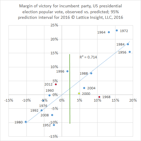
The results of the model are shown in the graph above. The horizontal axis represents the predicted margin of victory for the incumbent party, and the vertical axis represents the actual margin of victory. The closer the points are to the diagonal line, the more accurate the predictions. In fact, for this model, R-squared is 0.714, a strong correlation.
Indeed, the ultimate outcomes are predicted correctly 14 out of 16 times, for the presidential elections from 1952 to 2012. The correctly predicted elections appear in the upper right and the lower left. The exceptions, to the upper left and the lower right, are shown in red. In 1968, the election should have been won by Hubert Humphrey based on economic data, but perhaps due to the vast social turmoil that year, voters elected Richard Nixon. In 2012, the election should have been lost by Barack Obama based on economic data, but perhaps due to a weak campaign close by Mitt Romney, voters re-elected Obama.
The 2000 election appears in yellow. The model correctly predicts a popular vote victory by Al Gore, but this year was one of the rare times that the Electoral College vote was not consistent with the popular vote, and George Bush was elected.
Our model predicts that the Democrat nominee this year should have a 2.26% margin of victory in the popular vote over the Republican nominee. The 95% prediction interval gives a margin of error of plus or minus 12.5%. This interval is shown as a green line in the graph. The large margin of error is due in part to the small sample size (n = 16). An additional predictive variable might be helpful here, such as change in the crime rate or unemployment rate. In any case, we are 95% confident that the Democrat will win by up to 15%, or that the Republican will win by up to 10.5%. We'll talk again after the election!
I was curious to see if the national popular vote in the presidential election could be predicted on the basis of certain quantifiable variables. There is an adage that voters consider pocketbook issues foremost. I conjectured that the simplest variable affecting a voter's sense of economic health would be percent change from a year ago in real disposable income per capita. Disposable income refers to income after taxes; real means that this amount is adjusted for inflation; and per capita means averaged for every member of the population.
We consider this variable in three quarters prior to the general election, to help us predict the outcome. The outcome in this case is the percent margin in the national popular vote accruing to the party that currently holds the White House at the time of the election. The theory is that a larger increase in disposable income would be positively associated with support for the incumbent party.
The results of the model are shown in the graph above. The horizontal axis represents the predicted margin of victory for the incumbent party, and the vertical axis represents the actual margin of victory. The closer the points are to the diagonal line, the more accurate the predictions. In fact, for this model, R-squared is 0.714, a strong correlation.
Indeed, the ultimate outcomes are predicted correctly 14 out of 16 times, for the presidential elections from 1952 to 2012. The correctly predicted elections appear in the upper right and the lower left. The exceptions, to the upper left and the lower right, are shown in red. In 1968, the election should have been won by Hubert Humphrey based on economic data, but perhaps due to the vast social turmoil that year, voters elected Richard Nixon. In 2012, the election should have been lost by Barack Obama based on economic data, but perhaps due to a weak campaign close by Mitt Romney, voters re-elected Obama.
The 2000 election appears in yellow. The model correctly predicts a popular vote victory by Al Gore, but this year was one of the rare times that the Electoral College vote was not consistent with the popular vote, and George Bush was elected.
Our model predicts that the Democrat nominee this year should have a 2.26% margin of victory in the popular vote over the Republican nominee. The 95% prediction interval gives a margin of error of plus or minus 12.5%. This interval is shown as a green line in the graph. The large margin of error is due in part to the small sample size (n = 16). An additional predictive variable might be helpful here, such as change in the crime rate or unemployment rate. In any case, we are 95% confident that the Democrat will win by up to 15%, or that the Republican will win by up to 10.5%. We'll talk again after the election!
 RSS Feed